This is a preprint of an article accepted for publication in "Integrated Human Brain Science," ed. T. Nakada, Elsevier, 2000.
Independent Component Analysis of Simulated ERP Data
Scott Makeig1
scott@salk.edu
Tzyy-Ping Jung4
jung@salk.edu
Dara Ghahremani2
dara@salk.edu
Terrence J. Sejnowski2,3,4
terry@salk.edu
1
Naval Health Research CenterCurrently
The Salk Institute
La Jolla CA
2
Howard Hughes Medical InstituteComputational Neurobiology Laboratory
The Salk Institute
P. O. Box 85800
San Diego, CA 92186-5800
3
Department of BiologyUniversity of California San Diego
La Jolla, CA 92093
4
Institute for Neural ComputationUniversity of California San Diego
La Jolla, CA 92093
May10, 1999
This report was supported in part by the Navy Medical Research and Development Command and the Office of Naval Research, Department of the Navy under work unit ONR.Reimb-6429. The views expressed in this article are those of the authors and do not reflect the official policy or position of the Department of the Navy, Department of Defense, or the U.S. Government. Approved for public release, distribution unlimited.
A recently-derived infomax algorithm for performing Independent Component Analysis (ICA) (Bell & Sejnowski, 1995) is a new information-theoretic approach to the problem of separating multichannel electroencephalographic (EEG) or magnetoencephalographic (MEG) data into temporally independent and spatially stationary sources (Makeig et al., 1996). In a previous report, we have shown that the algorithm can separate simulated EEG source waveforms (independent simulated brain source activities mixed linearly at the scalp sensors), even in the presence of multiple low-level model brain and sensor noise sources (Ghahremani et al., 1996). Here, we demonstrate the ability of the ICA algorithm to decompose brief event-related potential (ERP) data sets into temporally independent components (Makeig et al., 1997) by applying it to simulated ERP-length EEG data synthesized from 3-sec (600-point) electrocorticographic (ECoG) epochs recorded from the cortical surface of a human undergoing pre-surgical evaluation (Bullock et al., 1995a, 1995b).
Six asynchronous single-channel ECoG data epochs were projected through single- and multiple-dipole model sources in a three-shell spherical head model (Dale & Sereno, 1993) to six simulated scalp sensors to create simulated EEG data. In two sets of simulation experiments, we altered relative source strengths, added multiple low-level sources (synthesized from ECoG data and uniform- or Gaussian-distributed noise), and permuted the simulated dipole source locations and orientations. The algorithm reliably separated the activities of the relatively strong sources, regardless of source location, dipole orientation, and low-level source distributions. Thus, the ICA algorithm should identify relatively strong, temporally independent and spatially overlapping ERP components arising from multiple brain and/or non-brain sources, regardless of their spatial distributions. When same simulated EEG data were decomposed using PCA, with or without Varimax and Promax rotation, the resulting component time waveforms were markedly less correlated with the time waveforms of the original sources than the ICA components.
The second simulation showed that the ICA algorithm can decompose ERPs generated by temporally uncorrelated sources. A third ERP simulation tested how the algorithm treated a simulated ERP epoch constructed using model ERP generators whose activations were partially correlated. In this case, the algorithm parsed the simulated ERP waveforms into a sum of temporally independent and spatially stationary components reflecting the changing topography of correlated source activity in the simulated ERP data. Each of the affected components sums activity from one or more concurrently-active brain generators. This suggests the ICA algorithm may also be useful for identifying event-related changes in the correlation structure of either spontaneous or event-related EEG data. Paradoxically, adding four simulated "no response" epochs to the training data minimized the relative importance of partial correlations in the original data epoch and allowed the algorithm to separate the concurrently active sources. Likewise, submitting ERPs from more than one stimulus or experimental condition to concurrent ICA analysis may allow the algorithm to separate sources from brain generators whose activations are partially correlated in some but not all response conditions.
Introduction
Event-related potentials (ERPs) are averages of electroencephalographic (EEG) epochs time-locked to a set of similar experimental events. Multichannel electromagnetic recordings from the scalp, including spontaneous EEG or magnetoencephalographic (MEG) records as well as ERP or magnetic event-related field (ERF) averages, have been widely used to study dynamic brain processes involved in perception, memory, selective attention, recognition, and priming. However, the combination of underlying brain processes that produce both spontaneous and event-related potentials and magnetic fields recorded at the scalp is still largely undetermined. Separating ERP sources without a priori knowledge of their number and spatial distribution is called a problem of "blind separation." Since ERPs often sum a complex distribution of activity in overlapping projections from brain and extra-brain generators to the scalp, it is difficult to identify and measure activity arising from each of the contributing sources. Mathematically, the inverse problem of identifying the locations and time courses of activation of brain generators of observed surface potentials is underdetermined. Most existing techniques for attempting ERP source separation employ second-order statistical methods (e.g. covariance, cross-correlation, and principal component analysis) (Chapman & McCrary, 1995), or else assume that sources have a known single- or multiple-dipole architecture (Scherg & Von Cramon, 1986).
Independent Component Analysis (ICA) algorithm we use here (Bell & Sejnowski, 1995) is a blind separation technique based on information-maximization which takes into account higher-order statistical information about the distribution of the input vectors (concurrent field measurements at many spatial locations). Recently, we have shown that the ICA algorithm can also be used to parsimoniously decompose brief ERP data sets into conventional ERP components (Makeig et al., 1997) (e.g., single peaks in the scalp waveforms, eye-movement activity, and steady-state responses (Pantev et al., 1993; Galambos, Makeig & Talmachoff, 1981)), spatially filtering each into a different output channel. Unlike algorithms that seek to both identify and localize ERP sources, the ICA algorithm does not attempt to perform three-dimensional source localization. Instead, it attempts to find the scalp topography of each source and the time course of its activation.
Without prior knowledge of the actual brain source activations that produce ERPs, it is difficult to verify the algorithms effectiveness. We assume there may be a few strong sources active during given ERP recording epochs, summing with activity generated by a larger number of weaker sources including residual spontaneous EEG sources not time- or phase-locked to the experimental events of interest. To determine whether the ICA algorithm can successfully separate relatively strong ERP components even when mixed with numerous weaker components, we performed several simulation experiments. These complement analyses of much longer (79,000-point) simulated EEG records performed previously (Ghahremani et al., 1996).
The simplest models of ERP generation assume that electrodes placed on the scalp surface record the electromagnetic activity of local or distributed cortical neural networks that can be modeled as effective single- or multiple-dipole sources (Nunez, 1981; Scherg & Von Cramon, 1986; Chapman & McCrary, 1995). Here, we simulate the activities of six simulated EEG components using ERP-length signals projected through a three-shell spherical head model to six model scalp electrodes (Dale & Sereno, 1993) and apply the ICA algorithm to the resulting simulated EEG data. These simulations allow us to investigate changes in ICA algorithm performance with variations in source strength, location, and orientation as well as effects of adding multiple weak EEG sources to the simulated EEG. We use simulated source data drawn from electrocorticographic (ECoG) data collected from the surface of the cortex of a patient undergoing exploratory analysis prior to surgery for epilepsy (Bullock et al., 1995a, 1995b). ECoG data epochs drawn from different channels and time periods in the available data set are used to simulate brief ERP-length EEG components. Further simulations, using artificial component waveforms resembling those produced by ICA decomposition of actual ERPs, clarify differences between ICA decomposition and physical source localization.
Figure 1
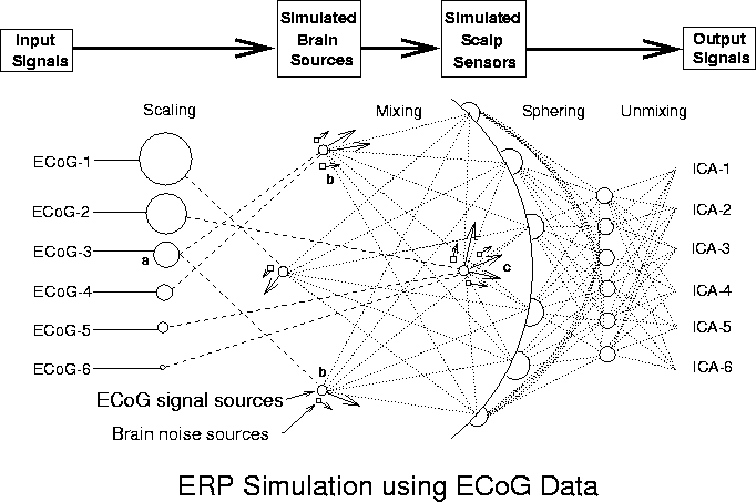
Figure 1. Schematic overview of the simulations. Input signals (ECoG-1 to ECoG-6), minimally correlated (|r| < 0.085) 600-point data epochs taken from different times and channels in an available ECoG data set were scaled relative to one another (Scaling) and assigned to single- or multiple-dipole brain sources (longer arrows). In some conditions, one source signal (a) was projected through bilateral dipole sources (b) approximately simulating a bitemporal source in the auditory cortices. Other signals were assigned to sources modeled as single dipoles with different orientations at the same brain location. Six weak ECoG (noise) sources (shorter arrows) were positioned near the seven signal dipoles. After initial "sphering" of the simulated ERP data, source separation was performed via the "unmixing" matrix produced by the ICA algorithm. Spatial filtering of the sphered simulated ERP data by multiplying with the unmixing matrix produced output component activation waveforms (ICA-1 to ICA-6).
Methods
An overview of the process of simulation and ICA decomposition is given in Figure1. The ICA algorithm is described in detail elsewhere. Further details and references about the algorithm and its application to EEG data appear in (Bell & Sejnowski, 1995; Ghahremani et al., 1996; Makeig et al., 1997; Jung et al., 1998; Jun et al., 1999; Makeig et al., 1999). Other related approaches and background material are available in (Cover, 1991; Linsker, 1992; Nadal & Parga, 1994; Jutten & Herault, 1994; Amari, Cichocki & Yang, 1996; Cardoso & Laheld, 1996; Karhumen et al., 1997; Lee, 1998).
The Three-shell Spherical Head Model
In our simulations, we use a three-shell spherical head model which projects dipoles at four fixed brain locations onto six scalp electrodes. The projection matrix containing the model parameters is computed using an analytic representation for a three-shell spherical head model (Dale & Sereno, 1993; Kavanaugh et al., 1978) as described in Appendix I.
Input Signals
The input signals are six asynchronous 3-sec (600-point) epochs of ECoG data drawn from different channels of a 12-minute, 80-channel ECoG data set (Bullock et al., 1995a) on the basis of being minimally correlated with one another. To simulate sources of varied strengths, in a second set of simulations we scale the input source signal vectors in steps of -3 or -6 dB relative to one another. Simulated ERP-length EEG signals are then derived from the input signals by multiplying by a mixing matrix specifying the projection of each model dipole to each model sensor.
Additional Low-Level Sources
In a second simulation, six additional simulated brain sources are added to the original six ECoG sources to produce simulated ERP-length EEG epochs. In one condition, these sources consist of ECoG data epochs uncorrelated with each other or with the first six ECoG source signals (|r| <=0.022). In other conditions, the low-level source waveforms are synthesized from uniform- or gaussian-distributed white noise. The low-level sources simulate weaker ERP components or residual EEG activity remaining in an ERP after finite averaging. The low-level sources are scaled to -3 or -6 dB below the level of the weakest ECoG signal source, and are then projected through simulated "diffuse" dipoles nearby the stronger source dipoles to the six simulated scalp electrodes. The "diffuse" dipole sources are modeled by adding 1% gaussian white noise to the weights in the mixing matrix specifying the projections of the strong sources to the model electrodes. In a third simulation, the orientations of the dipoles for the strong and low-level sources are independent of each other. In each condition, the mixed projections of the six weak and six stronger source signals are summed to form the simulated EEG data.
ICA Training
Training input consisted of 600 six-channel simulated EEG waveforms. The time order of the input data was reshuffled before each learning step to avoid overlearning. Training block length was 12. The initial ICA learning rate (0.006) was reduced by 15% after each training step when the change in the weight matrix (considered as a 1x36 vector) formed a greater than 90 deg angle to the weight vector change at the previous training step. Training was continued for at least 1024 steps to insure convergence.
Performance Measures
We measured the performance of the ICA algorithm by the correlations between source and output waveforms, and by the difference in maximal signal-to-noise ratio (SNR) of each input signal in the simulated EEG and ICA output data. These SNR measures are described in detail in Appendix II.
Simulations
1. ICA Decomposition is Independent of Source Projections

Figure 2a
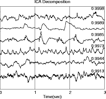
. ICA decomposition of simulated brief EEG data epochs derived from six 3-second (600-point) ECoG data epochs drawn from different times and channels in a 12-minute ECoG data set (a) and simulating the activities of six independent brain ERP sources.
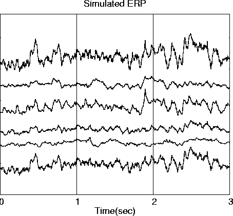
Figure 2c
. Projecting this source data through six one- and two-dipole simulated sources in a 3-layer spherical shell head model (c)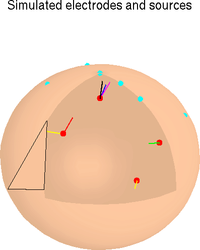
Figure 2b
. produces this simulated 600-point EEG data epoch.
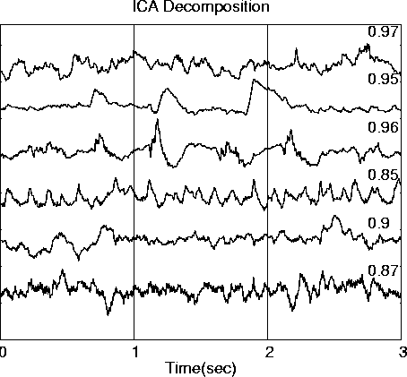
Figure 2d
. ICA decomposition of this data epoch produces six ICA component waveforms (d). Correlations between each ICA component waveform and its best-correlated input source waveform are shown on the right side of (d).To demonstrate the ability of ICA to unmix ERP-length data epochs, we first performed ERP simulations using six 600-point (3-sec) ECoG data epochs (Fig. 2a) drawn from different times and channels in a 12-minute ECoG data set (Bullock et al., 1995a, 1995b). The source epochs were selected as minimally correlated with each other (|r| <= 0.085). These source signals were projected through a mixing matrix representing 7 dipolar sources in the three-shell spherical brain model (Fig. 2c). One source projected to two dipoles with simulated bitemporal placement. The resulting simulated EEG scalp waveforms (Fig. 2b) were relatively highly correlated with one another (|r| = 0.24-0.98), and moderately correlated with the input source waveforms (|r| < 0.68).
Results
The ICA decomposition of the simulated ERP data is shown in Fig. 2d, with the maximal correlations between each ICA output waveform and its best-matching source waveform. These correlations are high in all cases (|r| > 0.87), but are less than unity because the input source waveforms are not truly independent.
Figure 3
|
|
|
|
|
|
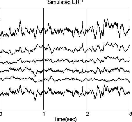
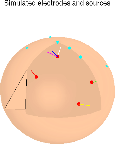
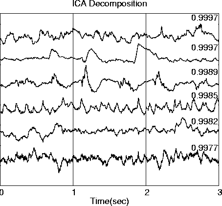
Fig. 3, gives results of a second simulation using the same source waveforms (Fig. 3a) with different dipole assignments and dipole angles (Fig. 3c), producing simulated ERP data (Fig. 3b) only moderately correlated with the simulated ERP data in the first simulation (Fig. 2b). Nevertheless, the ICA decomposition of the second ERP data set (Fig. 3d) is nearly identical to the ICA decomposition of the same data in the first simulation (Fig. 2d, |r| > 0.997).
Figure 4
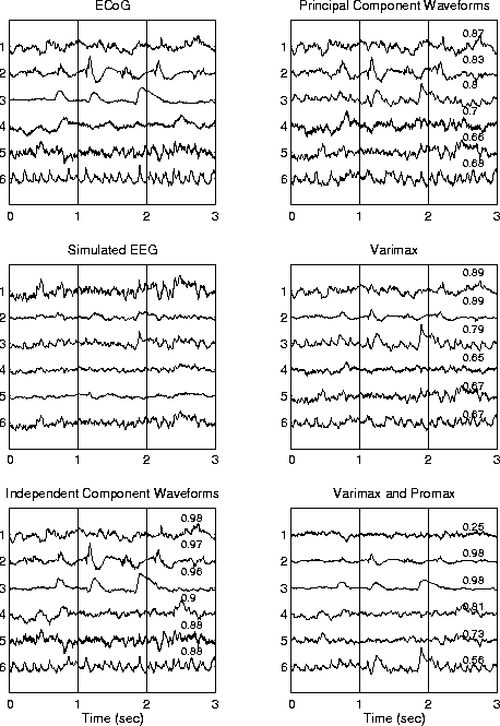
Figure 4 shows results of PCA-based decompositions of the same simulated data (middle left). PCA itself (upper right) rotates the first component so as to account for maximum variance in the data. This may sum activity produced by several independent components when these are spatially correlated. Succeeding principal components are both spatially and temporal uncorrelated with preceding components. Therefore, PCA itself is unable to separate sources whose projections to the scalp are spatially correlated. Mean absolute correlation of the 6 PCA component waveforms with the original source waveforms was 0.76. Varimax rotation is an orthogonal rotation method that attempts to minimize the number of temporal or spatial dimensions each component is weighted on. Varimax rotation (middle right) also gave a mean absolute correlation of 0.76. Promax is a constrained non-orthogonal rotation method that further concentrates large weights for each component on a few dimensions. Applied to the Varimax-rotated components (lower right), Promax produced two components (second and third from top) whose time waveforms were well-correlated (0.98) with two of the source waveforms (upper left). However, the mean absolute correlation for all six sources was only 0.72, well short of the 0.93 mean correlation for the ICA decomposition (lower left).
Figure 5
A further demonstration of the invariance of the ICA decomposition from source and sensor placements is the fact that the ICA decomposition of the original source vectors themselves, before mixing (Fig. 5), is nearly identical (|r| > 0.991) to the previous decompositions.
Conclusions
First, the ICA algorithm can reliably decompose six-channel, 600-point simulated (noise-free) ERP data sets into independent components. This was a remarkable result, since we assumed that the algorithm required much more input data to converge reliably because of its derivation from information theory. Recent work deriving the algorithm from maximum likelihood principles supports its use on shorter data epochs (Amari, Cichocki & Yang, 1996). Further, our results were obtained using ECoG waveforms recorded directly from the human cortical surface. Presumably, the dynamics and statistical distribution of ECoG data is as near to actual EEG source data as possible.
Second, the results of ICA decomposition do not depend on the mixing matrix, so long as it is non-singular. Singularity cannot be expected to be an issue in applications to real data since the inevitable presence of low-level and recording noise sources make non-singularity highly unlikely.
2. ICA Isolates Strong Signal Sources
When the total number of sources is larger than the number of data channels, changes in source location and orientation can produce large changes in the amplitude of the relative projections of different sources to the scalp, and thus possibly affect the ICA decomposition. To test this, we performed several simulation experiments decomposing simulated ERP-length data synthesized from more sources than the number of model sensors. These tested the ability of the ICA algorithm to accurately decompose simulated ERP-length EEG data even when it summed activity from more low-level sources than the number of simulated data channels.
Six new 3-sec ECoG data epochs, selected to be minimally correlated with each other and with the six epochs used in the first simulation, were used to simulate low-level ERP sources. In actual ERP data, these low-level sources might be either small ERP components or residual spontaneous EEG sources remaining in the data after finite averaging. In these simulations, the six stronger sources were scaled relative to one another before being assigned to model sources (cf. Fig. 2c) and projected via a mixing matrix to the six model scalp electrodes. In the first simulation, the attenuation step size was -6 dB, meaning these sources were scaled -6, -12, -18, -24, and -30 dB below the strongest source. The six additional low-level sources were scaled -36 dB below the strongest source, and were then projected through diffuse dipoles nearby and nearly parallel to the stronger source dipoles (Fig. 1). In another condition, different dipole assignments and orientations were used for the stronger and low-level sources.
Simulated 3-sec EEG epochs summing the stronger and low-level source projections were submitted to ICA decomposition. In each simulation reported below, 50 permutations of input signal attenuation order and model source assignment were used to produce 50 different input data sets. These were then decomposed separately using the ICA algorithm. Mean output SNR for each input source was then plotted as a function of the number of ICA training steps. In each simulation, the ICA algorithm was trained for 16,384 training steps to test for maximum convergence.
Results
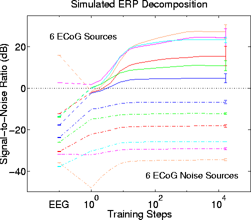
Fig. 6 shows SNR for the six stronger sources and six low-level sources before, during, and after ICA decomposition. Before training, only the two strongest sources have a positive SNR in any of the simulated scalp channels. After as few as 16 ICA training steps, all six sources are assigned to separate output channels with positive SNR. Output SNR is maximized after about 1000 training steps. Mean dB gain for the six stronger sources is 24 dB. The low-level sources are each largest in the same ICA output as their nearby stronger source, but in each case the SNR difference between the stronger and associated low-level source pairs is larger in the ICA output than in the simulated EEG input data. Effects of permuting the order of attenuation and source assignments are small, as shown by the (<= 3 dB) standard deviations across the 50 permutations (Fig. 6 right).
Figure 7a
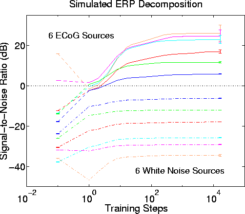
Figure 7a
. Invariance of the ICA decomposition to changes in low-level source distribution. Blind separation performance by infomax ICA using uniformly-distributed white noise for the six simulated low-level sources instead of ECoG data. Other parameters as in Fig. 6. Results strongly resemble results of simulations using 12 ECoG data sources (Fig. 6).Figure 7b
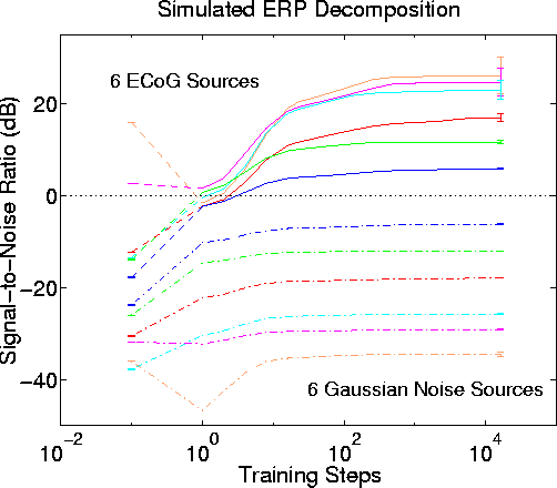
Figure 7b.
Blind separation performance by infomax ICA using Gaussian-distributed white noise for the six simulated low-level sources instead of ECoG data. Other parameters as in Fig. 6. Results again strongly resemble those using 12 ECoG data sources (Fig. 6).Fig. 7 shows the quite similar results of two more experiments in which (Fig. 7a) uniformly-distributed or (Fig. 7b) gaussian-distributed white noise were used instead of ECoG data to create the time waveforms of the six low-level sources. The similarity of the results in all three experiments implies that the statistical distributions of the low-level source strength values do not have important effect on the performance of the algorithm.
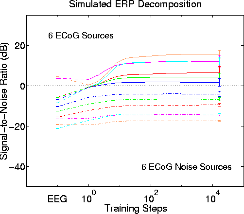
Figure 8.
ICA decomposition performance with stronger low-level sources. Blind separation performance by infomax ICA using -3 dB attenuation steps instead of -6 dB steps. Results of 50 simulations using different permutations of input signal order and source assignment. Other parameters as in Fig. 5. Again, the six largest input sources (solid lines) are assigned to different output components, and the output SNR order and range generally reproduce the order and range of source signal attenuation values. SNR gains (from best scalp channel to best output component) ranged from 8 dB to 21 dB (mean, 12 dB). The six lower-level sources (dashed lines), here scaled to -18 dB below the strongest source, have largest SNR in the same output component as their nearly larger source (shown by corresponding trace colors). Output SNR difference between the six stronger and low-level source pairs is 2 dB to 13 dB larger than in the simulated scalp data (mean, 7 dB).Fig. 8 shows parallel results of another simulation using a -3 dB source attenuation step size and ECoG source data. Again, all six stronger sources are separated into different ICA output channels with positive SNR, with somewhat lower final SNR values than the previous simulations using a -6 dB step size (here, mean SNR gain is 12 dB as compared to 14 dB in the first simulations).
Figure 9ab
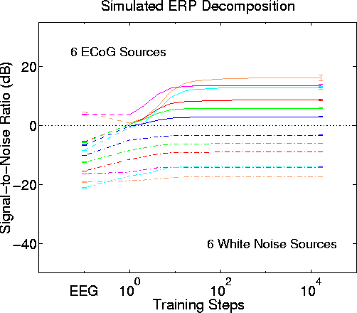
Figure 9a.
Invariance of the ICA decomposition to changes in low-level source distributions. Blind separation performance by infomax ICA with attenuation step size -3 dB and using uniformly-distributed white noise for the six simulated low-level sources. Other parameters as in Fig. 8. Results strongly resemble those in Fig. 8 using 12 ECoG data sources.
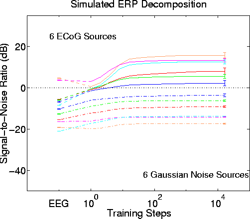
Figure 9b.
Blind separation performance by infomax ICA with attenuation step size -3 dB and using Gaussian-distributed white noise for the six simulated lower-level sources. Other parameters and results as in Fig. 8.Fig. 9 shows the very similar results of simulation experiments using either separate uniformly-distributed (Fig. 9a) or gaussian-distributed (Fig. 9b) white noise epochs to create the low-level source waveforms.
In Figs. 6 through 9, the low-level sources were nearby and near-parallel to the stronger source dipoles. Fig. 10
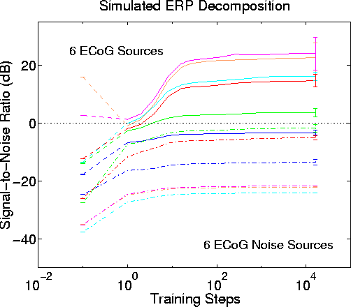
Figure 10.
Blind separation performance by infomax ICA with different dipole orientations for the stronger and low-level model source models. Results of 50 simulations using different permutations of input signal order and model source assignment. Signal attenuation step size is -6 dB. The six low-level EcoG sources (dashed lines) are assigned to the physical model sources shown in Fig. 3b, while the six stronger sources (solid lines) are assigned to model sources shown in Fig. 2b. After 16 training steps, five of the six strong input sources are assigned to different ICA components. SNR gains (from best scalp channel to best output component) ranged from 7 dB to 30 dB (mean, 25 dB), comparable to the SNR gains using in earlier simulations using model sources for the low-level inputs near those of the stronger inputs (Fig. 6).shows mean results of 50 simulations in which the source dipoles for the stronger and low-level sources were differently oriented. In this simulation, the attenuation step size was -6 dB and the low-level sources were ECoG data epochs. The source configurations of the stronger and low-level sources were those shown in Figs. 2c and 3c. Although in this case only the strongest 5 sources were separated by the algorithm into different output sources with positive SNR, mean SNR gain for the six stronger sources ranged from 7 dB to 30 dB (mean, 25 dB), quite comparable to earlier results (Fig. 6) using nearby dipole models for the low-level sources. Repeating this simulation using gaussian white noise instead of ECoG data epochs for the low-level sources produced nearly identical results (not shown).
Conclusions
The performance of the ICA algorithm in decomposing linearly-mixed simulated ERP-length EEG data sets degrades gracefully in the presence of additional low-level sources. The degree of separation achieved by the algorithm (measured here in terms of output SNR) depends on the relative amplitudes of the strong and low-level sources, and is weakly affected by their relative placements and orientations.
3. ICA Identifies Spatial Correlations in the Data
For most brain researchers, prototypical brain activity sources are active foci located in single brain structures. It is natural to ask, therefore, how the ICA algorithm treats data generated in several brain structures whose activations are partially correlated in time, since by definition Independent Component Analysis assumes its ICA sources are temporally independent. Brain generators whose activities are partially correlated cannot be independent sources of EEG or ERP data. How, then, does the ICA algorithm decompose their activities?
Fig. 11 (below) shows a simulation using six synthetic, partially-correlated simulated brain generator waveforms resembling ICA components produced when the algorithm was applied to actual auditory ERP data. Each simulated generator waveform is plotted as two 310-point response epochs. Note that the period of activation of generator 3 subsumes the activations of generators 1 and 2 (producing overall pairwise correlations of r= -0.460 and r= -0.128, respectively). These correlations were introduced deliberately to test the response of the ICA algorithm to correlated generator input. Other pairs of generator waveforms are nearly uncorrelated (|r| <= 0.070). The three waveforms (1-3) roughly simulate an extended activation (3) in one brain structure during which two other brain structures (1 and 2) briefly become active.
Results
Figure 11a
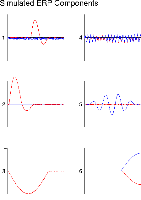
Figure 11a
. ICA decomposition of simulated partially-correlated source activity (b), synthesized by projecting the six synthetic 620-point brain-generator waveforms (a) through the dipole source model of Fig. 2a. Data are plotted as two 310-point waveforms. Note that time period of activation of source 3 overlaps those of sources 1 and 2..
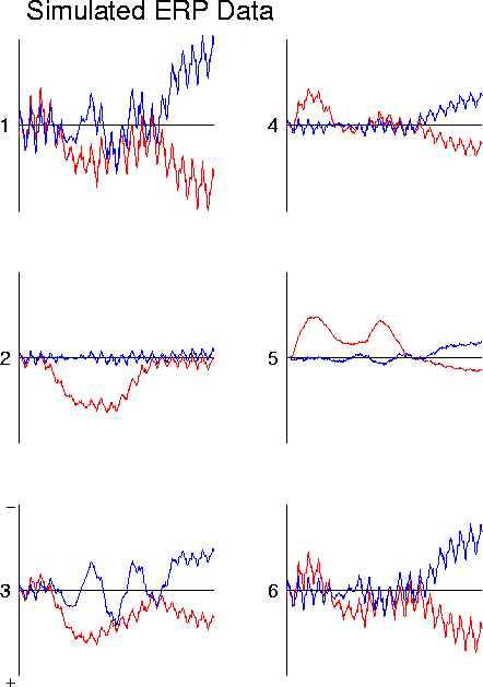
Figure 11b
. ICA decomposition of simulated partially-correlated source activity (b), synthesized by projecting the six synthetic 620-point brain-generator waveforms (a) through the dipole source model of Fig. 2a. Data are plotted as two 310-point waveforms. Note that time period of activation of source 3 overlaps those of sources 1 and 2.
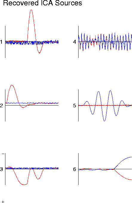
Figure 11c
. ICA decomposition of simulated partially-correlated source activity. Results of ICA decomposition of the simulated ERP wave forms are shown in (c). The time courses of activation of each source (except source 3) are returned by the algorithm.
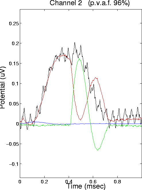
Figure 11d.
ICA decomposition of simulated partially-correlated source activity Plot (d) shows the results of projecting ICA sources 1, 2, and 3 onto simulated ERP channel 2. The simulated ERP waveform for channel 2 is also shown (note polarity change from (b).The three ICA components account for 96% of the variance in the simulated ERP, and together parse the correlation structure of the simulated ERP data into spatially-stable periods of source coactivation. This may or may not be useful for physiological investigation, depending on whether or whether not the coactivations are functional or adventitious (see text).Projecting the six simulated generator waveforms through the dipole model shown in Fig. 2c produces the simulated ERP data shown in Fig. 11b. The six simulated ERP channel waveforms contain a wide variety of features that might puzzle a psychophysiologist studying them. The ICA decomposition of this simulated ERP data is shown in Fig. 11c. Note first that the algorithm produces ICA source waveforms very similar to those of generators 1, 2, 4, 5, and 6. However, that of ICA source 3 differs from the waveform of generator 3 in two important respectsduring the activation periods of sources 1 and 2, ICA source 3 is silent.
Essentially, the ICA algorithm parses the data into periods of stationary spatial correlation, creating three ICA source components accounting for: (1) the activation of generator 3 alone, (2) the coactivation of generators 1 and 3, and (3) the coactivation of generators 2 and 3. The scalp projections of all three ICA sources, therefore, must also be composed of the scalp projection of generator 3, either alone or summed with the scalp projection of generator 1 or 2.
Fig. 11d shows the projections of ICA source components 1 to 3 onto model electrode 2, whose simulated ERP waveform is also shown. Three traces show the projections of ICA sources 1 through 3, respectively. Together, they sum to a waveform accounting for 96% of the variance in the model electrode response. (Remaining variance is explained by the other three ICA source components).
The infomax algorithm parses its input data into the sum of spatially stationary and temporally independent source activations. The decomposition produced by the ICA algorithm reveals, in this case, either: (1) the presence of functional coactivations of generator 3 and generators 1 and 2, (2) coactivations produced in the three generators by some other physiological source, or (3) adventitious correlations with little or no functional significance.
If the correlations in this simulation were indeed functional correlations, the ICA decomposition would actually be more physiologically informative than the physical generator decomposition given in Fig. 11a. The physical generator waveforms only show the time course of activation of the separate brain generators, ignoring their functional relationship, whereas the ICA algorithm parses the data into transient functional units defined by coactivation.
However, it is equally possible to imagine that the event-related coactivations of generators 1, 2, and 3 might be adventitious rather than a result of functional neural cooperativity. In this case, the ICA decomposition (Fig. 11c) would have less physiological significance than the physical generator decomposition (Fig. 11a). The three ICA source components in Fig. 11d each combine the activity of one or two generators (Fig. 11a), with generator 3 common to all the sources. Unfortunately, since the source inversion problem is underdetermined, no algorithm exists that can reliably determine the physical generator waveforms from the simulated scalp data alone.
Note that each ICA source in this simulations is spatially stationary and contains the activity of only one or at most two strong dipoles. This suggests that the ICA decomposition may be a useful preprocessing step prior to applying guided source inversion algorithms that attempt to solve the inverse problem using simplifying assumptions about the number and arrangement of dipolar sources present in the data (Scherg & Von Cramon, 1986; Dale & Sereno, 1993).
Although the ICA algorithm fits a linear model, ICA training is not a linear process. Fig. 12 shows the result of decomposing a data set in which four additional 620-point (no response) epochs of low-level (0.04 RMS) gaussian white noise
Figure 12
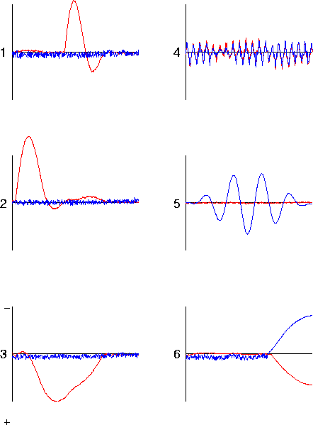
Figure 12
. Effects of additional simulated 'no-response' data on the ICA decomposition. ICA decomposition of a simulated ERP data set composed of five consecutive 620-point epochs. The first epoch was identical to that shown in Fig. 11b. The remaining four no response epochs were the result of projecting low-amplitude (0.04 RMS) white noise through the same dipole model of Fig. 2c. The 5 simulated response epochs were decomposed simultaneously by infomax ICA. The figure shows the first 620 points of the resulting ICA component waveforms. Note that the ICA component-3 waveform now follows the source-3 time course (Fig. 11a) more closely (see text).
were concatenated onto the simulated ERP data epoch of Fig. 11a. The figure shows the first epoch of the ICA source waveforms for the extended data set. The additional degrees of freedom in the appended no response data allows the algorithm to more closely approximate the actual activation time courses of all three generators (Fig. 11a).
Conclusions
Infomax ICA may fail to separate physically separable brain generators when their periods of activation are highly overlapping and input data length is short. In this case, the source decomposition produced by ICA will be physiologically significant only if the correlated activity in fact arises from transient functional correlations between them. The ICA algorithm parses the correlation structure of its input data into spatially stationary and minimally-correlated pieces, and when possible assigns each piece to a different output channel.
Anatomic considerations suggest that sensory and cognitive ERPs may be produced largely by sequences of brief activations in different neural networks. Our simulations suggest the ICA algorithm may be used to measure the latency, time course, spatial pattern, and strength of these activations, which may correspond to stages of neural information processing. ICA may be most useful when trained simultaneously on ERP data from several stimulus and/or task conditions, since in this case brief activations with different strengths and/or latencies in different response epochs are more likely to be minimally correlated. This hypothesis is supported by successful results of applying the ICA algorithm to several ERP data sets consisting of 2 to 64 related multi-channel waveforms (unpublished).
General Discussion
The reported effectiveness of the ICA algorithm in separating multiple linearly-mixed simulated audio and EEG sources (Bell & Sejnowski, 1995; Bell & Sejnowski, 1996) has been reproduced in ERP-length EEG simulations using a three-shell head model and six simulated scalp channels, in which stronger 600-point simulated-ERP signals generated from actual ECoG data epochs were successfully and repeatedly separated with SNR gains averaging 18 dB. Results were independent of the orientation or relative positions of the model dipole sources. As we have seen in decompositions of much longer simulated EEG data epochs (Ghahremani et al., 1996), the performance of the ICA algorithm degrades gracefully in the presence of multiple weak independent sources even when the total number of sources is larger than the number of sensors, and is relatively unaffected by source or sensor placements.
That an algorithm based on entropy maximization can be so efficient when given as few as 600 input vectors appears remarkable. Nonetheless, the simulations reported here, as well as recent theoretical work (Lee, 1998), plus published and unpublished results of applying the algorithm to several actual 14- to 128-channel ERP data sets, all imply that the ICA algorithm can correctly decompose ERP data of this complexity into a relatively small number of strong, spatially-stationary sources each accurately separating the correlated activations of one or more physical brain or extra-brain generators.
There is no universal definition of what constitutes an ERP component or source. Most researchers in the field believe that ERPs are composed largely of sequences of brief activations in different brain structures at different times relative to the time locking experimental events (see Makeig et al., 1977). These activations may overlap in time and their projections to the scalp sensors nearly always overlap spatially because of the spatial smearing of EEG signals produced by the high resistivity of the skull. Because waveforms containing single brief activations may be minimally correlated, ICA may be well-suited to ERP decomposition. In fact, our ICA decompositions of several ERP data sets also consist largely of brief sequences of separate source activations lasting 50-300 ms (Makeig et al., 1997; Makeig et al., 1999).
Results of our last simulation (Fig. 12) suggest the possible advantage of applying the ICA algorithm concurrently to ERP data from several stimulus and task conditions. In this case, the overall correlation induced by coincidental coactivations of pairs of sources in some but not all response conditions is lessened. Residual EEG and extra-brain noise in ERP signals may also be used by the algorithm to separate partially correlated but functionally independent sources (as in Fig. 12).
Conclusions
Infomax ICA is a promising tool for the analysis of multichannel EEG or MEG signals. Our results suggest that relatively strong brain source components may be effectively separated from each other and from weaker sources by ICA decomposition with SNR gains above 20 dB. ICA attempts to describe what independent sources produce its input data, as defined by their time courses and scalp maps, but not where in the brain the sources are located. It is thus compatible with the well-established indeterminacy of the source inverse problem. As the algorithm identifies sources by their spatial correlation structure, neurophysiological interpretation of ICA sources poses both research challenges and opportunities. The neurophysiological importance of transient event-related correlations in the activity of otherwise independent neurons and neural networks is now being studied seriously by theorists and experimentalists. Our simulations suggest the ICA algorithm may be a useful tool for identifying and monitoring spatiotemporal patterns of emergent correlation in brain activity linked to perceptual and cognitive brain processes.
Applications of ICA algorithm to averaged event-related potentials (ERPs) appear quite promising, since response averaging increases the amplitudes of activity time- and phase-locked to experimental events relative to the strength of other spontaneous and ongoing EEG sources. The number of independent strong brain sources contributing to ERP data thus may be smaller than the number of EEG channels typically used to record them (Makeig et al., 1997, 1999). In this case, the ICA algorithm should successfully separate and identify the time courses and scalp projections of the strongest ERP sources. ICA decomposition may be particularly useful for comparing the latencies, time courses, scalp topography, and activation strength of numerous brain generators involved in producing evoked responses to more than one stimulus in multiple experimental and task conditions.
Acknowledgements
This report was supported in part by grants to S.M., T-P.J. and T.J.S. from the Office of Naval Research, and to T.J.S. from the Howard Hughes Medical Institute. The authors wish to thank Anders Dale for supplying the head model parameters, Dr. Susan Spencer, Dr. Brad Duckrow, and Ted Bullock for supplying data used in the simulations, and Tony Bell for assistance and useful discussions.
References
Amari S., Cichocki, A. Yang, H.H. A new learning algorithm for blind signal separation. In Advances in Neural Information Processing Systems 8, MIT Press (1996).
Bell, A.J., Sejnowski, T.J. An information-maximization approach to blind separation and blind deconvolution, Neural Computation 7, 1129-1159 (1995).
Bell, A.J., Sejnowski, T.J. Learning the higher-order structure of a natural sound. Network: Computation in Neural Systems 7, 2 (1996).
Bullock, T. H., McClune, M. C., Achimowicz, J. Z., Iragui-Madoz, V. J., Duckrow, R. B. Spencer, S. S. EEG coherence has structure in the millimeter domain: subdural and hippocampal recordings from epileptic patients. Electroencephalograph. Clin. Neurophysiol. 95, 161-77 (1995a).
Bullock, T. H., McClune, M. S., Achimowicz, J. Z., Iragui-Madoz, V. J., Duckrow, R. B. Spencer, S. S. Temporal fluctuations in coherence of brain waves. Proc. Nat. Acad. Sci. USA 92 , 11,568-72 (1995b).
Cardoso, J-F. Laheld, B. Equivalent adaptive source separation. IEEE Trans. Signal Proc. 45:434-444 (1996).
Chapman, R.M. McCrary, J.W. EP component identification and measurement by principal components analysis. Brain and Language 27, 288-301 (1995).
Comon, P. Independent component analysis, a new concept? Signal Processing 36, 287-314 (1994).
Cover, T.M. Thomas, J.A. Elements of Information Theory, John Wiley (1991).
Dale, A.M. Sereno, M.I. Improved localization of cortical activity by combining EEG and MEG with MRI cortical surface reconstruction - a linear approach. J. Cogn. Neurosci. 5, 162-176 (1993
Galambos, R., Makeig, S. Talmachoff P. A 40 Hz auditory potential recorded from the human scalp. Proc. Natl. Acad. Sci. USA 78, 2643-2647 (1981).
Ghahremani, D,. Makeig, S., Jung T-P., Bell, A.J., Sejnowski, T. S. Independent Component Analysis of Simulated EEG Using a Three-Shell Spherical Head Model Technical Report INC-9601, Institute for Neural Computation, University of California San Diego. La Jolla CA (1996).
Jung, T-P., Colin Humphries, Te-Won Lee, Scott Makeig, Martin J. McKeown, Vicente Iragui, Terrence J. Sejnowski. "Extended ICA Removes Artifacts from Electroencephalographic Recordings" In: D. Touretzky, M. Mozer and M. Hasselmo (Eds). Advances in Neural Information Processing Systems 10:894-900 (1998).
Jung, T-P., Makeig, S., Westerfield, M., Townsend, J., Courchesne, E., and Sejnowski, T. J., "Analyzing and Visualizing Single-trial Event-related Potentials," In: Advances in Neural Information Processing Systems 11 (1999, in press).
Jutten, C. Herault, J. Blind separation of sources, part I: an adaptive algorithm based on neuromimetic architecture. Signal Processing 24, 1-10 (1991).
Karhumen, J., Oja, E., Wang, L., Vigario, R. Joutsenalo, J. A class of neural networks for independent component analysis. IEEE Trans. Neural Networks 8:487-504 (1997).
Kavanagh R.N., Darcey T.M., Lehmann D., Fender D.H. Evaluation of methods for three-dimensional localization of electrical sources in the human brain. IEEE Trans. Biomed. Eng. 9, 25:421-429 (1978).
Lee, Te-Won, Independent Component Analysis: Theory and Applications, Boston: Kluwer Academic Publishers (1998).
Linsker, R. Local synaptic learning rules suffice to maximise mutual information in a linear network. Neural Computation 4, 691-702 (1992)
Makeig, S., Anthony J. Bell, Tzyy-Ping Jung and Terrence J. Sejnowski, "Independent component analysis of electroencephalographic data," In: D. Touretzky, M. Mozer and M. Hasselmo (Eds). Advances in Neural Information Processing Systems 8:145-151 (1996).
Makeig, S. Tzyy-Ping Jung, Anthony J. Bell, Dara Ghahremani, Terrence J. Sejnowski, "Blind Separation of Auditory Event-related Brain Responses into Independent Components," Proc. of National Academy of Sciences, 94:10979-84 (1997).
Scott Makeig, Marissa Westerfield, Tzyy-Ping Jung, James Covington, Jeanne Townsend, Terrence J. Sejnowski and Eric Courchesne, "Functionally Independent Components of the Late Positive Event-Related Potential during Visual Spatial Attention," J. Neurosci. 19:2665-2680 (1999).
Nadal, J-P. Parga, N. Non-linear neurons in the low noise limit: a factorial code maximises information transfer. Network 5, 565-581 (1994).
Nunez, P.L. Electric Fields of the Brain. New York: Oxford (1981).
Pantev, C., Elbert, T., Makeig, S., Hampson, S., Eulitz, C. Hoke, M. Relationship of transient and steady-state auditory evoked fields. Electroencephalogr. Clin. Neurophysiol. 88, 389-396 (1993).
Scherg, M. Von Cramon, D. Evoked dipole source potentials of the human auditory cortex.
Electroencephalogr. Clin. Neurophysiol., 65, 344-60 (1986).
Appendix I
Details of the Simulations
The three-shell spherical head model
In our simulations, we used a three-shell spherical head model which projects dipoles at four fixed brain locations onto six scalp electrodes. The projection matrix containing the model parameters was precomputed using an analytic representation for a three-shell spherical head model (Dale & Sereno, 1993; Kavanagh et al., 1976). Electrode positions were vertices of a triangulated icosahedron located on the model head sphere. At each of the four locations in the head model, we placed one to three dipoles pointing in different directions, giving a total of seven dipoles. We assigned five input signals to single dipoles, and one input signal to two bilateral dipoles (Fig. 2c). As shown in Fig. 2c, two dipoles with different orientations were placed at a single dipole location, and three dipoles with different orientations were placed at another location.
These choices were expressed via a ((4x3)x6) configuration matrix, C, which assigned six source signals to the seven dipoles according to the configuration described above. The configuration matrix was then multiplied by the (6x(4x3)) weight matrix, F, which projected the seven dipoles (at the four dipole locations) to each of the six simulated electrode sites. The resulting matrix product:
![]()
was a 6x6 "mixing" matrix specifying the simulated EEG signals as linear combinations of the six input sources. Simulation variables were chosen such that this mixing matrix was non-singular. Note that despite the complexity of the head model, the mixing matrix was a linear 6x6 transformation of the six sources, and therefore satisfied the assumptions of the algorithm.
Source strength adjustment
To simulate sources with varied strengths, the vector of input signals, s(t), were scaled relative to one another in steps of -6 or -3 dB using a 6x6 diagonal attenuation matrix, . Simulated EEG signals, A, were derived from the input signals by multiplying by the attenuation and mixing matrices.
![]()
Weak brain sources
In some experiments, seven simulated weak brain source signals were added to the simulated EEG. These ("brain noise") sources consisted of uncorrelated random noise with a flat distribution in the [-1,1] interval, scaled to the same level as the weakest input source signal. The seven brain noise sources were assigned to simulated "diffuse" dipoles placed nearby each of the seven brain source dipoles by adding 1% gaussian-distributed noise to the matrix, M, before mixing. The mixed brain noise signals were then added to the simulated EEG.
Appendix II
Separation Performance Measures
SNR in the ICA algorithm output
Our measure of the ICA algorithms performance in these simulations is the signal-to-noise ratio (SNR) of each input signal in the output sources. For each input signal, si(t), we defined:
![]()
in which all input signals except for si(t) were zeroed out. The output source waveforms for si(t) were then defined as:
![]()
The signal level, SikICA, of the ith input signal in the kth output source waveform was computed by taking the standard deviation of the kth row of ui(t). The noise level for each input signal in each output source was computed by letting sic(t) consist of all input signals except si(t):
These "complementary" signal vectors were passed through the simulated mixing and unmixing processes with brain noise and sensor noise sources added, giving output source waveforms:
![]()
where n(t) is the weak brain sources and r(t) is the sensor noise. The noise level, NikICA(t) , was defined as the standard deviation of the kth row of uic(t). Then, the SNR of the ith signal in the ICA algorithm source waveforms was defined as:
![]()
where n is the number of sources.
SNR in the simulated EEG
The SNR of each input signal in the simulated EEG was computed for comparison with [] the SNR in the ICA output. The signal level, SijEEG, for the ith input signal in the simulated EEG signal was defined as the standard deviation of the simulated EEG in the jth recording electrode (i.e. in the jth row of xi(t)):
![]()
The noise level, NijEEG, for the ith input signal was defined as the standard deviation of the jth row of the complementary mixed signal matrix:
![]()
The SNR of the ith input signal in the simulated EEG was then defined as:
![]()
where m is the number of sensors.
SNR gain from EEG to ICA algorithm outputs
For each input signal, the difference between its SNRICA and SNREEG was defined as the SNR gain, G, resulting from ICA algorithm source separation.
![]()